Why Chinese say maybe and but
I watched a TED recently that Sarah Jones(a actress) played the role of 11 people from different cultures to response to random questions asked by TED audiences.
I was impressed by the Chinese American woman she played who always repeat “BUT” and “Maybe”. It heard like a typical Chinese speaker. I began to think why Chinese people tend to say these two words again and again. One reason is that they are not good at express themselves. The second reason might be they are not confident; they feel insecurity. She said that at least the food should not be poison. As you know, food, sex and sacurity are the basic needs of human according to Maslow’s hierarchy of needs.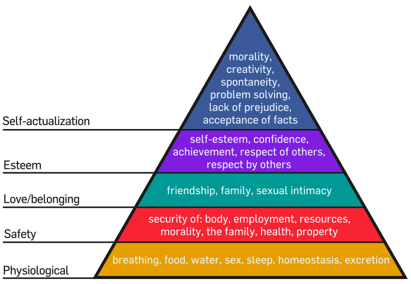
Why Chinese people are lack of sacurity. Well, it is a long story. To make it brief—it is becuase poisonous food, polluted air and water, dominated culture and so on. A survey report that many rich people in China want to imgrant to other country such as US, Canada. Some Corrupt officials want to have orther country’s identity because they want to escape from the punishment. There also a lot of people want to go US, becuase they worry about the nature and social environment, they worry about the education and healthy of their children.
Lost in local extrema
I love this place, the library at the second floor in Aderhold Building. I love this table, which is not too big but just enough. This love can guide me back home.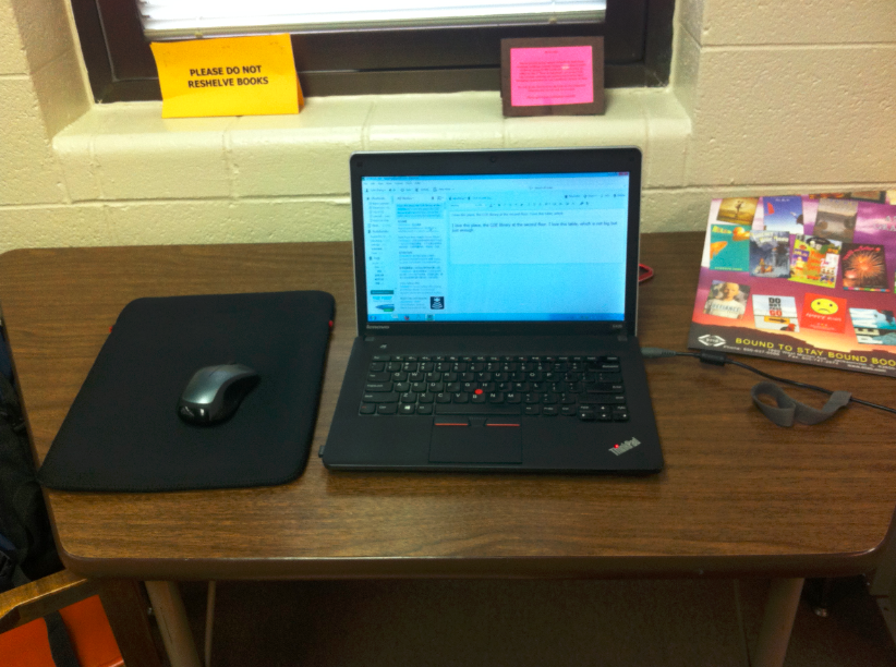
I lost myself sometimes in some very narrow area. People may ignore the whole when they are attracted and trapped by them. It can be power, It can be sex, It can also be anger and violence.
A picture comes to my mind when I am thinking of these dangerous Local Extrema—the local extrema. I frist notice this phenomenion in NG’s machine learning class. This is the picture that he used to show local extrema.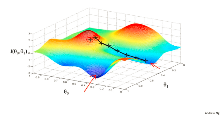
When the computer only have one seed, it is very likely trapped in a local extrema and return a wrong answer. It is just like a person who lost himself when he try to reach the extrema unrealized that it is only the local extrema.
R语言学习笔记
##week1
getwd() #获取当前工作目录
setwd(dir) #设定当前工作目录 也可以直接通过菜单界面设定
source("myfunction.R") #加入源之后才可以使用这个函数

##week2
#list
> a <- 1:10
> b <- c(1,3,4,5,8,9,11,14,15,18)
> b <- b[-2] #去除第二个元素
> c(1,2)*c(2,3)
[1] 2 6

> m <- c(1,2,3)
> mynames <- c("1-2","2-3","4-5")
> mytable <- setNames(m,mynames)#之后可以通过name来调用元素值
1-2 2-3 4-5
  1   2   3

> union(x, y) #并集
> intersect(x, y) #交集
> setdiff(x, y) #前者有后者没有的
> setequal(x, y) #元素是否全部相同
> is.element(el, set)
> unlist() #将层级list变为单层
> unique(x) # 获取非重复元素

# logical operation
x <- FALSE
y <- TRUE
! x
x & y
x && y
x | y
x || y
xor(x, y)

isTRUE(x)
cbind(a,b) #
rbind(a,b) #
length(a) #
class(a)
as.character()
as.logical()
as.numeric()
m <- matrix(a,nrow=2,ncol=5)
dim(m) #[1] 2 5
attributes(m) $dim [1] 2 5
m <- 1:10
dim(m) < c(2,5) #
f <- factor("yes","no","yes","yes")
table(f) # yes 3 no 1
x <- c()
x <- c(x,1)
mean() #求平均值
cor(a,b) #求相关系数
is.na()
is.nan()

## file 文件
read.table() #读取txt表格
read.csv() #读取csv文件
# 写文件略过row name
write.csv(data, "data.csv", row.names=FALSE)
# 同样写文件,当用空白替换"NA"
write.csv(data, "data.csv", row.names=FALSE, na="")
# 使用tabs略过row col name
write.table(data, "data.csv", sep="\t", row.names=FALSE, col.names=FALSE)
参考[Cookbook for R » Writing data to a file](http://www.cookbook-r.com/Data_input_and_output/Writing_data_to_a_file/)
write.table(sim, "pcksim.csv", row.names=na,col.names=c("",na),sep = ",") # 可以写列名称

names()
x[!is.na(x)] # 去除缺失的数据
data <- data.frame(id=1:10,height=170:180)
data["id"] #返回局部data.frame
data["id"][!is.na(data["height"])] #返回height无缺失的id
data[[id]] #返回vector
paste("00","1",".csv",sep="") # 001.csv
paste(a,collapse="") # 将一个list连成一个长字符

for (i in 1:length(id)){
    s <- as.character(id[i])
    spre <- paste(rep("0",3-nchar(s)),collapse="") # use collapse join vector
    fn <- paste(directory,"/",spre,s,".csv",sep="") # use sep to join string
    data <- read.csv(fn)
}

if(length(x)>0){print(x)}else{}

##Week3
x <- list(a=1:5,b=rnorm(10))
lapply(x,mean)#$a[1] 3  $b[1] 0.03937816
如果x不是一个list,那么它将被自动转换成list,相当于使用as.list()函数
x <- list(a=matrix(1:4,2,2),b=matrix(1:6,3,2))
lapply(x,function(elt)elt[,1]) #$a[1] 1 2  $b[1] 1 2 3
lapply(x,function(elt) strsplit(elt,"-")) #对每个元素使用“-”进行拆分
sapply(x,mean) #会自动简化结果,返回一个vector或者matrix,不能简化返回list
x <- matrix(rnorm(200),20,10)
apply(x,2,mean) #返回10列的均值
apply(x,1,sum) #返回每行的总和共20个
a <- array(rnorm(2*2*10),c(2,2,10)) #三维数组
apply(a,c(1,2),mean)
          [,1]      [,2]
[1,] 0.1888774 0.5517366
[2,] 0.2667046 0.2412767

str() #Compactly Display the Structure of an Arbitrary R Object
str(tapply)
> x <- c(rnorm(10),runif(10),rnorm(10,1))
> f <-gl(3,10) #生成标签 1 1 1 1 1 1 1 1 1 1 2 2 2 2 2 2 2 2 2 2 3 3 3 3 3 3 3 3 3 3
> tapply(x,f,mean) #具有相同标签的数值的平均值
with(mtcars, tapply(mpg, cyl, mean))# mtcars is a data.frame with cyl and mpg

> split(x,f) #利用标签将list进行拆分
> s <- split(airdata, airdata$Month)
> lapply(s,function(x) colMeans(x[,c("Ozone","Solar.R","Wind")]))
split(x,list(f1,f2),drop=TRUE) # empty levels can be dropped

## 字符串 string
> as.character()
> strsplit("1-2,3-4,5-6",",") #对字符串进行拆分
> strsplit("1-2,3-4,5-6",",")[[1]][1] #返回 "1-2"
> paste(rev(strsplit("abc", split = "")[[1]]), collapse = "") #反转字符串
> grep("bcd", "abcd") # return 1 #
> regexpr("bcd","aabcd")
[1] 3
attr(,"match.length")
[1] 3
attr(,"useBytes")
[1] TRUE

> gregexpr("1","1-2,2-3,1-5") #返回所有匹配位置 也能利用length获取匹配数目
> length(gregexpr("1","1-2,2-3,1-5,1-9,1-8")[[1]]) #返回4


> mapply(rep,1:4,4:1)
[[1]]
[1] 1 1 1 1

[[2]]
[1] 2 2 2

[[3]]
[1] 3 3

[[4]]
[1] 4

## debug
traceback() # print out where error occurs,else do nothing
debug() # step through one line at a time
browser() #suspend the execution wherever called and put it in debug mode
trace() # insert debug code in specific place

#Play with the iris data
library(datasets)
data(iris)

#Play with $
> x <- makeCacheMatrix()
> x
$set
function (y)
{
    x <<- y
    inv <<- NULL
}

$get
function ()
x

$setinverse
function (inverse)
inv <<- inverse

$getinverse
function ()
inv

> x$set(matrix(rnorm(9),3,3))
> x$get()

> x$set(a)
> x$get()
            [,1]      [,2]       [,3]
[1,] -0.50184759 -0.751659 -2.1276852
[2,]  0.37466264 -1.448643  1.1807655
[3,] -0.06093845  0.740338 -0.8508723
> cacheSolve(x)
           [,1]       [,2]       [,3]
[1,] -0.4668678  2.8847043  5.1705844
[2,] -0.3214999 -0.3872940  0.2664879
[3,] -0.2462983 -0.5435808 -1.3137063

#week4
#统计
str(str)# see the structure of a object
m <- matrix(rnorm(100),10,10)
str(m)
str(lm)
str(ls)
x <- rnorm(100,2,4)
summary(x) #摘要
table(x) #返回频数表
str(x)

#作图
hist(rnorm(1000,2,4))
hist(BMI, breaks=20, main="Breaks=20")
hist(BMI, breaks=seq(17,32,by=3), main="Breaks is vector of breakpoints")
seq(0, 1, length.out = 10) #在一定范围产生制定数目的序列
plot(x,y)

#拟合
> set.seed(20)  #进而可以再次产生同样的随机数 方便别人重复模拟
> x <- rnorm(100)
> e <-rnorm(100,0,2)
> y <- 0.5+2*x+e
> sumary(y)

#评估运算时间 user time(cpu 时间消耗)elipsed time(流逝壁钟时间)
> system.time(readLines("http://www.jhsph.edu"))

#就
make.Negloglik <- function(data, fixed=c(FALSE,FALSE)){
    params<- fixed
    function(p){
        params[!fixed] <- p
        mu <- params[1]
        sigma <- params[2]
        a <- -0.5*length(data)*log(2*pi*sigma^2)
        b <- -0.5*sum((data-mu)^2)/(sigma^2)
        -(a+b)
    }
}
set.seed(1)
normals <- rnorm(100,1,2)
nLL <- make.Negloglik(normals)
optim(c(mu=0,sigma=1),nLL)$par

> # Fixing sigma=2
> nLL <- make.Negloglik(normals,c(FALSE,2))
> optimize(nLL,c(-1,3))$minimum
[1] 1.217775
> optimize(nLL,c(-1,2))$minimum
[1] 1.217775
> #Fixing u=1
> nLL <- make.Negloglik(normals,c(1,FALSE))
> optimize(nLL,c(1e-6,10))$minimum
[1] 1.800596
> nLL <- make.Negloglik(normals,c(1,FALSE))
> x <- seq(1.7,1.9,len=100)
> y <- sapply(x,nLL)
> plot (x,exp(-(y-min(y))),type="l")
> nLL <- make.Negloglik(normals,c(FALSE,2))
> x <- seq(0.5,1.5,len=100)
> y <-sapply(x,nLL)
> plot(x,exp(-(y-min(y))),type="l")


Assignment 3
#在R中有的时候表达方式是不一样的,比如
引用某个变量的子变量用
time$year #而不是time.year

##常犯错误
该使用[]的时候错误的使用了(),特别是在操作data.frame的时候
该使用[[]]错误的使用了[],前者可以变为向量,后者还是data.frame
忘记了使用%%进行
判断是否包含
"a" %in% c("a","b","c")
表示数组相乘用
%*%

如何使用Order
> (ii <- order(x <- c(1,1,3:1,1:4,3), y <- c(9,9:1), z <- c(2,1:9)))
 [1]  6  5  2  1  7  4 10  8  3  9
 > rbind(x, y, z)[,ii] # shows the reordering (ties via 2nd & 3rd arg)
  [,1] [,2] [,3] [,4] [,5] [,6] [,7] [,8] [,9] [,10]
x    1    1    1    1    2    2    3    3    3     4
y    5    6    9    9    4    7    1    3    8     2
z    5    4    1    2    6    3    9    7    2     8
不同发电机的原理
原电池发电(化学能转化为电能)
以铜锌原电池为例,其中锌电极发生的电极反应式是:
锌片 Zn-2e-=Zn2+ (氧化反应)
锌离子进入溶液,使得溶液里的正电荷过多;同时锌失去的电子沿导线经电流计流入铜片,使溶液里原有的氢离子在铜电极上被还原成氢原子,这样溶液中多余的正电荷就被中和;氢原子又结合成氢分子并放出。铜电极发生的电极反应式是:
铜片 2H++2e-=H2↑ (还原反应)
由于在锌、铜两个电极上不断发生的氧化还原反应,使化学能转变为电能。锌片是给出电子的一极,是电池的负极,铜片是电子流入的一极,是电池的正极。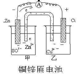
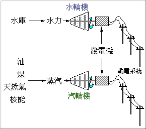
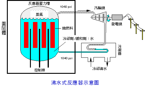
动力发电(水力、火力、风力、核能、太阳能蒸汽发电)
其原理是利用动力推动线圈切割磁感应线发电。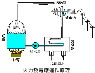
热电机
其原理是热电效应,即不同的金属导体(或半导体)具有不同的自由电子密度,当两种不同的金属导体相互接触时,在接触面上的电子就会扩散以消除电子密度的差异。而电子的扩散速率与接触区的温度成正比,所以只要维持两金属间的温差,就能使电子持续扩散,在两块金属的另两个端点形成稳定的电压。由此产生的电压通常每开尔文温差只有几微伏。如能适当设计和组合就可以产生工作电压。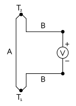
太阳能发电
其原理主要依赖于光电效应。
太阳光照在半导体p-n结上,形成新的空穴-电子对,在p-n结电场的作用下,光生空穴流向p区,光生电子流向n区,接通电路后就形成电流。这就是光电效应太阳能电池的工作原理。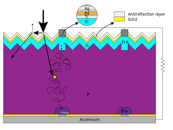
原电池反应_百度百科: http://baike.baidu.com/view/159629.htm
各种发电方式:http://vm.nthu.edu.tw/science/shows/nue/various.html
热电效应 - 维基百科:http://zh.wikipedia.org/wiki/%E7%86%B1%E9%9B%BB%E6%95%88%E6%87%89
Solar cell - Wikipedia:http://en.wikipedia.org/wiki/Solar_cell
Chinese Puzzle Pot design
There is an interesting class called Intro to the design of everything link here
They showed a pot that can put in water by a hole at the bottom, and no water come out. It works well.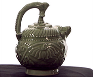
The following is one possible inner structure design in my mind.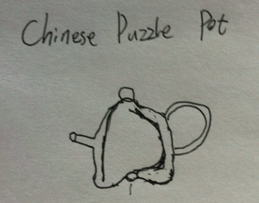
Repeated Measures Correlation Mixed Model
How to do it?
Analysis==>Mixed Model, then you got diaogue 1 as follows. ID shuold be put be included as subjects. Year should be included as repeated, cause I measured multiple times by different year.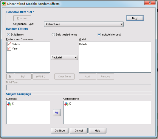
The most hard decision to make is which Repeated Covaricance Type to select, there are a lot of choices, the most used ones are:
- Unstructured: you have no idea of the correlation of repeated measures, SPSS we estimate all the correlation independantly (r12,r13,r23,r14,r24,r34).
- Scaled Identity: no correlations at all, r=0.
- Compound Symmetry: all correlations equals r.
- AR1: (r, r^2, R^3)
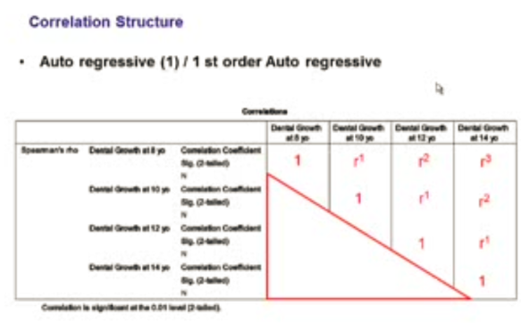
- Toeplitz:(a,a,a,b,b,c)

- Another choice is “diagonal” which assumes no correlation between the random effects.
Then you determing the fixed effect variable: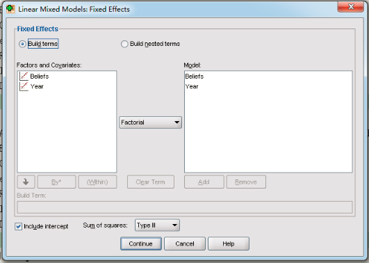
And the random effect variable: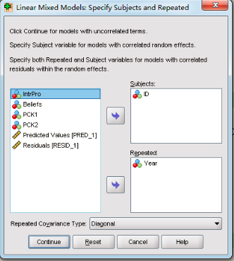
Ecojustice work
share a film clip that portrays an environemntal meassage
美丽的大脚
photo essay
sustainability share-a-thon
book study
nature principle presentation
memory banking
pick a community practice and interview some people who participate in this practice to grow your knowledge about this practice. I selected foot ball as both comercial and community practice. I wrote a post about foot ball.
Citizen Science
Citizen science (also known as crowd science, crowd-sourced science, civic science, or networked science) is scientific research conducted, in whole or in part, by amateur or nonprofessional scientists, often by crowdsourcing and crowdfunding. Formally, citizen science has been defined as “the systematic collection and analysis of data; development of technology; testing of natural phenomena; and the dissemination of these activities by researchers on a primarily avocational basis”.[1] Citizen science is sometimes called “public participation in scientific research.”[2]
[1] “Finalizing a Definition of “Citizen Science” and “Citizen Scientists””. OpenScientist. 2011-09-03. Retrieved 2012-10-11.
[2] Hand, E. (2010). “Citizen science: People power”. Nature 466 (7307): 685–687. doi:10.1038/466685a. PMID 20686547
from: wikipedia
多次重测数据的方差分析
统计学比较抽象,需要通过例子加以学习。
比如第一型错误(Type I error)和第二型错误(Type II error)。比如验证一个人的智商是否超常(极高或者极低),我们知道95%人群的智商在70-130之间,一般成正态分布。我们会做出一个零假设H0,假定某人的智商是正常的。然后用某种评估方法测量一个人的智商结果是145,超出正常范围,这样我们就否定零假设,认为该人智商是超常的。
但是我们的评估方法不一定准确,所以不可避免的会犯错误。第一型错误是,该人智商属于正常范围(接受H0),但是的统计评测显示的却是超常(拒绝H0)。第二型错误是,该人智商明明超常(拒绝H0),结果我们统计评测显示该人智商正常(接受H0)。简单说也就是假阳性和假阴性,或者假检出和假包含。
分析数据就像是在森林里寻宝,每次进入森林都很不容易,需要花很多时间,非常容易迷失方向,面对无数的表格和无数的可能分析方法不知所措。而且好不容要到的路径,下次再想用却忘记了,需要花费很多实践才能再次找到。于是很多人做了很多无用的功,就是在原地打转。为了避免这样的情形发生,分析数据时一定要写分析记录和报告,否则即便是文件夹里有无数的报表,也忘记当初这个报表是干什么的了。
如何使用SPSS绘制重复测量的误差条图?答案是可以使用SPSS的graph builder,不过我在用的过程中发现一个很低级的错误。我搜索到了一个视频教程Create a clustered bar or line chart of means for repeated measures data (with optional error bars) on Vimeo。其实原理很简单,就是把多个变量同时拉到纵轴。但是我拉的时候,系统却不容许,也不报错。晕。后来发现,原来这些变量必须是scale类型,而不能是normal。全部粘贴覆盖为scale之后,问题解决。不提示为什么不能拖拽,这是SPSS设计上的缺陷。其实类似的问题还有,当你使用Multiple Imputation(MI)处理缺失数据的时候,如果变量类型不是scale,SPSS也会拒绝执行MI,这也是在网上查了才解决的。因此,在使用SPSS的时候一定要小心的变量类型,尽量最开始就设好。
下面进入正题,如何进行重复测量的方差检验。其实如何做并不难,难的是如何解释Spss产生的一大推报表,并选择有用的信息进行报告。首先这样的检测一般可以分为两类:One Way Anova以及Two-way Anova。前者是单因素实验设计,后者是双因素实验设计(如V1(2)× V2(3)交叉设计,共有6组)。两者的区别以后再解释。
此外还有组间变量(比如不同的处理、教学方法、培训类型)和协变量(性别、教育程度)等。
这种统计方法往往可以让你检测是否存在交叉效应。
在报告的时候,SPSS同时给你multivariate test和Univariate test的结果。到底报告那个呢?取决于Mauchly’s Test of Sphericity,如果sig<0.05那么,说明球度(sphericity)假设不成立,那么就要看修正后的Univerite test的结果。Spss提供多个修正结果,根据Epsilon-Greenhouse-Geisser的值是否大于0.75进行不同的选择,如果大于则选择Huynh-Feldt修正的结果,否则则选Greenhouse结果。
另外就是如何报告F检验的结果。通常报告的格式如下F(自由度,误差自由度)=F值,p=sig,n=total。这些值在哪里呢?看下图。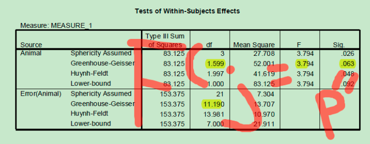
那么如何报告One way Anova的结果呢?
One way Anova
APA报告格式为:F(3,165)=2.836 p=0.04<.05
其中3为组间自由度(组数4-1),165为组内自由度(样本总数169-组数4)。所以看到这个结果,就知道共分4组,样本总量为169(3+165+1)。F值为2.836,p值为0.04,达到了显著水平。
NARST 2014 Pittsburgh
The National Association for Research in Science Teaching (NARST) is a worldwide organization of professionals committed to the improvement of science teaching and learning through research. More about NARST click here.

The 2014 Annual meeting is hold in Pittsburgh from March 30 to April 2. The theme of this meeting is “AWAKENING DIALOGUES — Advancing Science Education Research Practices and Policies”. I attended this conference and presented a paper with my advisor. There were more than one thousand of participants from more than 25 countries. And many many presentations and posters were going on at the same time. Fortunately I bought the conference program book which contain maps and all related information. Although I did take my laptop with me, but actually I found that the book helped me a lot especially on finding a place and planing for where to go in order to listen to special presentations.
There were 13 sessions in total. I attended 10 sessions and plus 1 session in which I presented our study on teacher perception. I arrived at Sunday afternoon and missed 2 sessions. But after that, I managed to took all the left sessions. So you can imagine how busy I was at that time when going from one room to another room. I thought we could not attend the committee meeting but in fact Dr Jackson told me we were allowed to do that as long as we were interested. Next time I would like to have a try. It was really a pity that I forgot to take a picture with my advisor. In fact I just took a lot of pictures of other researchers’ slides but did not take any picture of myself. Instead, my advisor took some pictures for me when I was introducing our study. During the last session, a presenter asked the audiences(only 3 people including me because most had left) to took a picture with her. This was the only picture that I took with others in my first NARST conferences. Next time I don’t want such a harry anymore. I will try to take my time to enjoy the next conference rather than keep running all the time.